Google Ads

Thursday, November 10, 2011

Hexagons, part I

We interrupt our regularly scheduled series to present to you the amazing hexagon.

Here is a regular hexagon:

clip_image001

You might say, “Tom, what’s so special about a hexagon?” Let me tell you:

  1. It has the most number of sides (6) of any regular polygon that can be tiled (there other polygons with more sides such as some decagons that can be tiled, but they won’t be “regular”).
  2. They have a very special relationship to circles, which I will get into at a later time.
  3. Hexagons appear in nature in many places and ways:
    1. A honeycomb is made of hundreds or thousands of hexagons;
    2. The north pole of Saturn has a hexagonal cloud pattern.
    3. Snowflakes have hexagonal crystal structures.

The fact of the matter is, hexagons appear in nature so much because they make efficient use of space.

Here’s an interesting fact about regular hexagons.  Let’s take a regular hexagon and draw a circle around it such that the vertices of the hexagon are all on the circle’s edge, like so:

clip_image001[1]

Let me tell you an interesting property of the hexagon in the above figure: the sides of the hexagon are all equal to the radius of the circle it inscribes!

So, we’re going to talk about hexagons a little.

Thursday, October 6, 2011

Differentials–The Elusive Concept?

A friend to Tom’s Math Class writes:
A while ago after I'd taken a few years of Calculus (nothing too advanced), I was frustrated at the vague and ambiguous definitions of "differentials" (dx, dy). I learned from the literature that it IS somewhat of an illusive concept.
Liz, NY
Ah, differentials.  Differentials can be somewhat elusive, though, it bothers me that you received “vague and ambiguous definitions,” because the term “differential” is exactly what it sounds like: a difference, in this case, the difference between two points on a curve that define a line.

We’re going to delve into some linear algebra here for a moment.  Take the following function:

f(x)=x2


If you were to graph out this function, you would get a specific curve called a parabola:
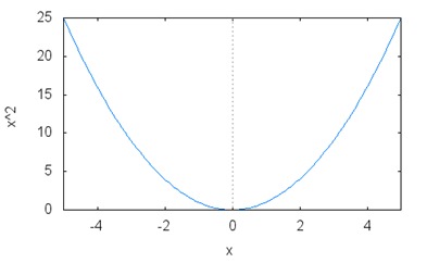
parabola plot

This parabola is the most basic curve in linear algebra, and it is usually the first introduced to students.  Now, differentials are about tangents to this curve, and this all has to do with speed and acceleration.  If the x axis represented time, and the y axis represented distance, then we could say that this curve could represent the distance traveled over time.

Let’s give a real world (okay, somewhat real world—all of the conditions presented here would have to be extreme circumstances, but I don’t make the rules) example to demonstrate what I mean.

Let’s pretend that we’re train engineers.  A mysterious set of circumstances have occurred to damage our speedometer but not our odometer.  We need to know what speed the train is travelling at any particular instant to know how much pressure to apply to the braking system.  We do have a stopwatch, so the instant we start moving, we start the stopwatch.  After 1 minute, we have gone 1 mile, so we write 1 min = 1 mile.  After 2 minutes, we’ve gone 4 miles.  After 3 minutes, we’ve gone 9 miles, and so on. 

You’ll notice that if d = distance in miles and t = time in minutes, then the distance travelled would have to be d = t2.  So how do we know the instantaneous speed at any time t?  Well, we could say that the average speed overall is 9 miles / 3 minutes = 3 miles per minute.  But that’s not the whole story.  If at minute 2 we’ve gone 4 miles and at minute 3 we’ve gone 9 miles then the average speed between minutes 2 and 3 is:

average speed over a minute

5 miles per minute average speed between minutes 2 and 3.  If you’ll notice, this formula is exactly the same as the formula for slope:

slope

Well, that’s because it is.  In linear algebra (and the calculus that springs from it), speed=slope.
So at the 3 minute mark, how fast are we really going?  Let’s look at a table of varying times that will get arbitrarily closer and closer to t = 3 minutes.

x2 x1 f(x2) f(x1) average speed
3 2.5 9 6.25 5.5
3 2.75 9 7.5625 5.75
3 2.85 9 8.1225 5.85
3 2.95 9 8.7025 5.95
3 2.975 9 8.850625 5.975
3 2.99 9 8.9401 5.99
3 2.999 9 8.994001 5.999
3 2.9999 9 8.9994 5.9999
3 2.999999 9 8.999994 5.999999


If you’ll notice, the closer x1 gets to x2, the closer the average speed gets to 6 but not quite.  Why?  Because there’s a problem in the formula used to determine this speed:

Average speed

If x2 ever equals x1, then the denominator in this formula becomes 0, a condition that is undefined and causes the universe to collapse into a massive black hole.

So let’s define a new variable: Δx (read “delta x”) and define Δx as being x2-x1.  And we also need something to stop Δx from becoming 0, thus saving the universe.  This is called a “limit,” and we symbolize it like this:

limits

And what we’re doing is getting the slope of the tangent of f(x) at an arbitrary point, so we’d symbolize that as:

dx dy f of x

So our new formula would look like this:

differential equation


Since we’ve defined f(x) as being equal to x2, let’s see how this plays out.
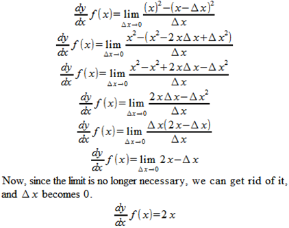
x squared derived

So, now we know exactly how fast our train is going at 3 minutes, and can verify that it is, indeed going 6 miles per minute, since x=3, and 2x=6.

To bring it back to the original question: a differential is defined specifically as follows:

A differential is the difference between two points on a curve, producing a slope.  As the differential approaches zero, the resultant slope gets closer to representing the slope of the tangent to the curve at a particular point.
In other words: Δx.

I know I’ll be laughed out of my Math Club, but I cannot recommend Calculus for Dummies by Mark Ryan enough.  It’s superbly written, and fully explains in plain English these concepts and many more.

Sunday, October 2, 2011

Symbolic Logic 3: The Or Operator

In the last post, we discussed the “And” operator (symbolized as “∧” as in “P ∧ Q”).  Today, we’re going to discuss its brother, “Or.”
Similar to the And operator, Or is symbolized thusly:
PQ
And just like And, an Or statement can be evaluated to True or False.  The difference with Or is that it evaluates to False only if both component statements are False.  Here is the truth table for PQ
P Q P Q
True
True True
True False True
False True True
False False False
The definition of the “Or” operator could be this:
The “Or” operator evaluates to False if and only if both component operands are False.
If you’ll recall, we had values for P and Q:
P=”The car is green”
Q=”The car has four doors.”
So PQ would read as:
Either the car is green or it has four doors, or both.
If our hypothetical car has two doors, this statement is still true, because both predicates must evaluate to False in order for the whole thing to be False.  In fact, let’s look at the truth table for this statement, just for fun:
Either the car is green or it doesn’t have four doors, or both.
That would be symbolized like this:
P~Q
Here’s the truth table of that statement:
P Q ~Q P~Q
True True False True
True False True True
False True False False
False False True True
This is interesting.  This statement seems to be false only if it has four doors, but it isn’t green.  Might there be a causal relationship here?  Let’s look at this another way.  Let’s say P=”The car is a coupe.” and Q=”The car is fast.”  P ∨ ~Q seems to imply that in order for you to have a fast car, it must be a coupe.  That seems to say something wholly different.  I’ll cover that in my next post.
Next: Differentials
Next in the Logic Series: The If… Then Operator

Friday, September 30, 2011

Symbolic Logic, Part II: The “And” Operator

In the last post, we discussed the statement P, which we defined as “The car is green,” and how the statement is either True, or it is False.  We also talked about “not P”, which we symbolized as ~P.

Now, let’s say we have another statement:
The car has four doors.
We’re going to call this statement Q. It also has two possible states: True and False. Here is its truth table:

Q

True

False

And here is the truth table for Q and ~Q:

Q ~Q
True False
False True

Now we can combine P and Q to create a compound statement thusly:

The car is green and it has four doors.

We are going to symbolize this conjunction like so:

PQ

That little upside-down “V” between P and Q represents the operator “and,” and the statement as a whole would be read “P and Q.” Now, PQ also evaluates as a whole statement to either True or False, but this depends on the values of both P and Q. In the case of the ∧ operator, both P and Q must be True for PQ to be True. Here is the truth table for this:

P Q PQ
True True True
True False False
False True False
False False False

So, if we say PQ, but the car actually has two doors, then it doesn’t really matter what color the car is, the entire statement is false.  The rule of the “And” operator is this:

A compound statement using the “And” operator evaluates to True if and only if both component statements are True; otherwise, the compound statement is False.

If we were going to say that:

The car is green and does not have four doors.

We would symbolize it thusly:

P ∧ ~Q

And the truth table would look like this:


P Q ~Q P ∧ ~Q
True True False False
True False True True
False True False False
False False True False

So, in the case of our hypothetical two-door, green car, P ∧ ~Q will evaluate to True, since it is true that the car is green and it does not have four doors.  Note that this statement is also True if the car has five doors, or three doors, or anything other than four doors.

Next: The “Or” Operator

Tuesday, September 27, 2011

Symbolic Logic, part I: Introduction to Basic Concepts

One important area of math is “symbolic logic,” which is also known as “formal logic” or sometimes “Boolean algebra.”
Here’s how it starts.  I’m going to start with a statement:
The car is green.
We are going to call this statement P.  Note that when we say “statement,” we mean something that is factual, not opinion.  So “The car is green” is okay (as long as we agree what “green” is: but, I digress), but “The car is beautiful” is not.  Our statement P can have one of two states: It can either be True or it can be False.  If we were to put these possible values into a table, they would look like this:
P
True
False
It may seem a bit silly to have such a table, but I’m introducing it here to introduce the concept of the “Truth table.” This is the truth table of the statement P.
Note that there is no “Maybe” listed here.  That’s because in logic, a statement is either totally true or it is totally false.  There is no middle ground; the car is either green or it is not.  If it’s “kinda” green, then it’s not green, and the statement would be false.  Now, we could get into arguments about the definition of “green,” and get into specific color wavelengths on the electromagnetic spectrum, but for our purposes, green is green, and a car is either green or it isn’t.
Then there is this statement:
The car is not green.
We could call this statement “not P.”  We would symbolize it thusly: ~P.  Whenever P is True, ~P is false, and vice versa.  The truth table would look like this:

P ~P
True False
False True
Next: We will be introducing compound statements.

Sunday, September 25, 2011

Fixing the Variance Percentage Program

Okay, the previous VBA function has a few flaws: it doesn’t test for empty cells, and it is rather inefficient when it comes to memory; it stores the results in an array.

For reference, here is the original code:

Public Function LowestCompPer(vRg As Range) As Double
Dim n As Integer
Dim t As Integer
Dim p() As Double
Dim i As Integer
Dim wsf As WorksheetFunction
Dim j As Integer
Dim k As Integer
Set wsf = Excel.WorksheetFunction
n = vRg.Count
t = (n * (n - 1)) / 2
ReDim p(t) As Double
k = 1
For i = 1 To n - 1
For j = i + 1 To n
p(k) = Abs(vRg(i) - vRg(j)) / (wsf.Max(Abs(vRg(i)), Abs(vRg(j))))
k = k + 1
Next j
Next i
Dim min As Integer
min = 1
For i = 1 To t
If p(i) < p(min) Then
min = i
End If
Next i
LowestCompPer = p(min)
End Function

Now we’re going to fix this.  Here we go:

Public Function LowestCompPer(vRg As Range) As Double
Dim i As Integer
Dim j As Integer
Dim k As Integer
Dim FullCells As New Collection
Dim PerDbl As Double
Dim min As Double
'get a count of how many cells aren't empty
'also keep a collection of cells that aren't empty
'This will kill two birds with one stone: it will allow us
'us to get rid of the triangular number calculation,
'as well as make sure that all cells we're referring to
'actually have values in them.
For i = 1 To vRg.Count
If vRg(i) <> "" Then
FullCells.Add vRg(i)
End If

Next i
'k keeps track of whether or not the first minimum has been calculation.
'0=no, 1=yes
k = 0
For i = 1 To FullCells.Count - 1
For j = i + 1 To FullCells.Count
'PerDbl temporarily stores the results of our comparison formula
PerDbl = Abs(FullCells(i) - FullCells(j)) / _
(Application.WorksheetFunction.Max(Abs(FullCells(i)), _
Abs(FullCells(j))))
'We have to start somewhere. Remember, all percentages will be
'positive
'Since min always start at 0, we have to initialize min
'Once we've done that, though, we don't want to change it
'again unless we've found a smaller number
If k = 0 Then
min = PerDbl
k = 1
ElseIf PerDbl < min Then
min = PerDbl
End If
Next j
Next i
'Never forget to clean up!
Set FullCells = Nothing
LowestCompPer = min
End Function


It may seem strange, but it works.  It may seem like we have traded one inefficiency (looping twice) with another (storing full cells in a Collection), but this was necessary to make sure that the entire range is full.

Leave any comments or questions you may have below.

Sunday, September 11, 2011

Variance Problem, Part 2: Electric Boogaloo


To continue from the last post:

Your boss approaches you.  He has a list of 40 SKUs that have been inventoried.  He says, “We need to adjust the inventory on these products.  Each of these SKUs has 4 counts associated with them.  This is represented on this list as the difference between what we actually have and what the computer is telling us we should have.  The only way we can adjust these is if two counts for each product agree with each other within 10%.  Find which ones can be adjusted, and make the appropriate adjustments.”

Here is the table with the SKUs and the four count variances per SKU:


SKU
Var 1
Var 2
Var 3
Var 4
00001
- 42
- 44
- 52
- 42
00002
- 80
-38
- 34
- 93
00007
- 11
+ 2
- 15
- 9
00013
- 85
- 131
- 51
- 74
00020
- 86
- 212
- 83
- 77
00028
- 99
- 202
- 157
- 88
00037
+ 92
+ 16
+ 46
+ 97
00040
+ 91
+ 191
+ 70
+ 82
00050
+ 12
+ 2
+ 18
+ 13
00060
+ 43
+ 48
+ 30
+ 44
00069
+ 31
+ 51
+ 39
+ 34
00074
- 57
- 105
- 70
- 50
00075
- 88
- 31
- 71
- 72
00077
+ 56
+ 104
+ 55
+ 53
00082
+ 68
+ 43
+ 69
+ 73
00090
- 29
- 62
- 26
- 32
00093
- 55
- 73
- 81
- 65
00098
- 34
- 17
- 28
- 32
00108
- 13
- 7
- 18
- 14
00109
- 40
- 7
- 59
- 44
00113
+ 42
- 11
+ 31
+ 39
00117
- 50
- 90
- 65
- 44
00124
- 40
- 92
- 61
- 34
00127
+ 87
- 13
+ 89
+ 97
00135
+ 91
- 10
+ 43
+ 102
00138
- 50
- 42
- 56
- 43
00141
+ 2
+ 0
+ 2
+ 2
00144
- 61
- 19
- 77
- 64
00152
- 5
+ 2
- 6
- 6
00162
+ 30
+ 44
+ 31
+ 28
00169
+ 15
+ 5
+ 22
+ 18
00173
- 66
- 111
- 35
- 58
00179
- 9
- 1
- 5
- 10
00189
- 36
- 2
- 52
- 39
00194
+ 89
+ 219
+ 114
+ 88
00202
- 49
+ 21
- 31
- 55
00212
- 89
- 146
- 95
- 100
00218
- 75
- 105
- 32
- 74
00223
- 78
- 179
- 83
- 63


If you remember the Variance Problem from the last post, you will remember that the formula to get the variance percentage looks a little something like this:


For each of these SKUs, this will have to be done 6 times (again, see the last post to see why).  That means we will have to do this calculation 240 times.  Woof.
Okay, so we do a macro.  We have several choices, here.


  1. We could have a macro that goes through each SKU one-by-one, does all of the calculations, and highlights the ones that are good.
  2. We could create a user-defined function that we could put into the “F” column to show the lowest variance percentage.

Since I like to show my work, I choose option 2.

First, I save this spreadsheet as an .xlsm file, so it can have macros in it.  Next, I go into the VBA editor (Alt+F11) and this is the formula I put into the editor:

Public Function LowestCompPer(vRg As Range) As Double
    Dim n As Integer
    Dim t As Integer
    Dim p() As Double
    Dim i As Integer
    Dim wsf As WorksheetFunction
    Dim j As Integer
    Dim k As Integer
    Set wsf = Excel.WorksheetFunction
    n = vRg.Count
    t = (n * (n - 1)) / 2
    ReDim p(t) As Double
    k = 1
    For i = 1 To n - 1
        For j = i + 1 To n
            p(k) = Abs(vRg(i) - vRg(j)) / (wsf.Max(Abs(vRg(i)), Abs(vRg(j))))
            k = k + 1
        Next j
    Next i
    Dim min As Integer
    min = 1
    For i = 1 To t
        If p(i) < p(min) Then
            min = i
        End If
    Next i
    LowestCompPer = p(min)
End Function

Here’s how it works.  First, an arbitrary number of cells get passed to the function (you in the back, be quiet—I'm getting to it, I promise). We need to know how many comparisons need to be made (t). Then we need to create a variable that will hold all of the calculations for us. It then goes through all of the necessary combinations and puts two numbers through our variance comparison formula and stores it in the p(k) array. Then, it goes through all of these results stored in the p array and determines the lowest (again, you in the back: BE QUIET) percentages. It then returns the lowest percentage.


What you do is you put the following in the “E” column:

=LowestCompPer(B2:E2)
After autofilling, you get something like this:


SKU Var 1 Var 2 Var 3 Var 4 Compare Percentage
00001
- 42
- 44
- 52
- 42
0%
00002
- 80
- 38
- 34
- 93
11%
00007
- 11
+ 2
- 15
- 9
18%
00013
- 85
- 131
- 51
- 74
13%
00020
- 86
- 212
- 83
- 77
3%
00028
- 99
- 202
- 157
- 88
11%
00037
+ 92
+ 16
+ 46
+ 97
5%
00040
+ 91
+ 191
+ 70
+ 82
10%
00050
+ 12
+ 2
+ 18
+ 13
8%
00060
+ 43
+ 48
+ 30
+ 44
2%
00069
+ 31
+ 51
+ 39
+ 34
9%
00074
- 57
- 105
- 70
- 50
12%
00075
- 88
- 31
- 71
- 72
1%
00077
+ 56
+ 104
+ 55
+ 53
2%
00082
+ 68
+ 43
+ 69
+ 73
1%
00090
- 29
- 62
- 26
- 32
9%
00093
- 55
- 73
- 81
- 65
10%
00098
- 34
- 17
- 28
- 32
6%
00108
- 13
- 7
- 18
- 14
7%
00109
- 40
- 7
- 59
- 44
9%
00113
+ 42
- 11
+ 31
+ 39
7%
00117
- 50
- 90
- 65
- 44
12%
00124
- 40
- 92
- 61
- 34
15%
00127
+ 87
- 13
+ 89
+ 97
2%
00135
+ 91
- 10
+ 43
+ 102
11%
00138
- 50
- 42
- 56
- 43
2%
00141
+ 2
+ 0
+ 2
+ 2
0%
00144
- 61
- 19
- 77
- 64
5%
00152
- 5
+ 2
- 6
- 6
0%
00162
+ 30
+ 44
+ 31
+ 28
3%
00169
+ 15
+ 5
+ 22
+ 18
17%
00173
- 66
- 111
- 35
- 58
12%
00179
- 9
- 1
- 5
- 10
10%
00189
- 36
- 2
- 52
- 39
8%
00194
+ 89
+ 219
+ 114
+ 88
1%
00202
- 49
+ 21
- 31
- 55
11%
00212
- 89
- 146
- 95
- 100
5%
00218
- 75
- 105
- 32
- 74
1%
00223
- 78
- 179
- 83
- 63
6%


Note here that there are some here that do not fit within the boss's requirements (for example: 00169) because none of the count variances are within 10%. Who did these counts, anyway?

A confession: This is not the optimal solution. The function stores the comparison percentage in an array, and it turns out the array is not necessary. I made this function in the heat of the moment after getting a project at work much like the one referred to here. Also, the function will throw an exception if it encounters an empty cell (since it is intended to be used in a cell, you will get a “#VALUE!” error).

Next, I'm going to show how to fix this to be more efficient and to be able to handle empty cells.